Online Stochastic Matching

In this post, I want to explain a bit about my research experience in Online Stochastic Matching. But as my research for this project is not finished yet, I will just explain the preliminaries of my research and the way I (as a junior researcher) look at these type of problems.

In 1990 Karp, and Vazirani and Vazirani published a paper called an Optimal Algorithm for on-line bipartite matching which introduces the ranking algorithm. They showed that their algorithm achieves (1-1/e) competitive ratio (comparing to offline version,) and no other algorithm can beat this ratio. This paper was a starting point for lots of future works. So it is useful to take a close look at their algorithm and ways to analyze it.

What is on-line Bipartite Matching?

There are different ways to introduce an on-line version of Bipartite matching. One of them is motivated by Internet advertising display applications. In this setting, users search for a keyword and the algorithm wants to match users to some relevant advertisers. The advertisers (left vertices) are known in advance and they just prefer to match to relevant users. Users (right vertices) arrive online as they search in the search engine. Upon their arrival, the algorithm should match one of the interested advertisers to the user (i.e. Display the corresponding ad) or ignore the users. In the original setting of Karp, Vazirani, Vazirani there was no priory assumption about the type of users and advertisers can have arbitrary any function for determining whether a user is relevant to them or not.

So here the challenge is that we need to choose a permanent action (matching) before knowing all information about the problem (just like any online algorithm problem). If we were allowed to change our past decisions, then on the arrival of each right node, we would be able to match optimally whether by matching it to a free neighbor or by just a chain of swapping of matched nodes. But now upon the arrival of each node, we need to match it permanently or leave it free.

A simple algorithm
Upon the arrival of each vertex, match it to its lowest index free neighbors if it has any.

This algorithm and any other algorithm that matches whenever it can (a maximal match), is always at least as good as half of the optimum offline solution (maximum-mal match). Because this statement is true for any two maximal matches. So we can simply achieve a 0.5 competitive ratio, but can we do better?

The adversary

To determine whether we can perform better than half, we need to think about the worst-case scenario for each algorithm that we want to analyze. It is useful to think about the worst-case as an adversary trying to bring us the worst-case instance. Here, it is crucial to define the strength and limitations of the adversary. We define three possible adversaries:

Strong adversary

This type of adversary is a bit stronger than usual adversary types but let’s define it for future discussion! This type of adversary needs to choose the number of left vertices at the beginning. Then the game starts. In each step, the adversary might add a new right node and identify its left neighbors or terminates the game otherwise. Upon the arrival of each node, the algorithm might match it or not. But based on her action, the adversary will do the next action. The adversary might end the game after any number of steps. Competing against this type of adversary to get a better competitive ratio than half is a hopeless job. Because this type of adversary is really strong as he can identify the neighborhood of each right node after observing the algorithm’s actions. For instance, the adversary can do the following strategy to get the half competitive ratio:
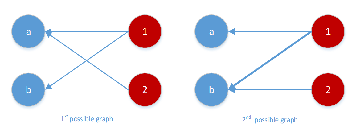
He chooses the number of left vertices to be 2 at the beginning and in the first step, he identifies the neighbors of the first right node as follows:

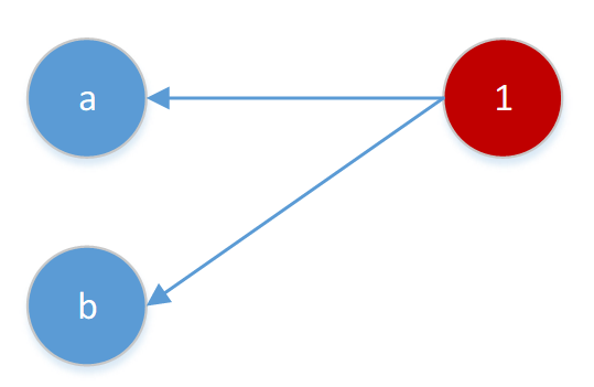
Based on the action done by the algorithm (which is shown by the orange arrow), the adversary will show one of the following neighbors for the next vertex.

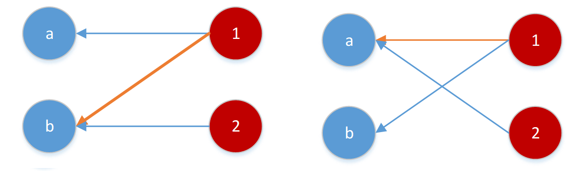
In any of these two scenarios, the second node cannot get matched. The adversary will terminate the game in this step. We left with one match while the off-line version for both graphs matches both right vertices. So the worst case competitive ratio is exactly half and not more. Therefore, to beat the half, we need to restrict the strength of the adversary.

Normal Adversary

This type of adversary is just the usual adversary. This adversary knows the algorithm that we are going to use at the beginning, he should identify the entire bipartite graph before the algorithm makes any decision. Here, if the algorithm is a deterministic one, the normal adversary is as strong as the stronger type of adversary as he can predict the actions done by algorithm precisely at the beginning and construct the bipartite graph accordingly. Therefore, we need to add randomness to our algorithm to have any chance of beating the half! We want to make an unpredictable algorithm to not allowing the normal adversary to act as a strong adversary.

Let’s try to find a good algorithm!

Ok. Let’s think about what we would expect from our algorithm in instances that have two left vertices and then try to generalize our strategy for any possible bipartite graph.
In the beginning, our algorithm sees the first vertex (call it “1”) and its neighbors that adversary designed for us. If “1” has a single neighbor, there is no harm to match it in any possible scenario so we expect our algorithm to match it. But if “1” has two neighbors (a and b), our algorithm should identify that with what probability we will match it to “a” ($p_a$ ) and or to “b ($p_b$ ). (There is no point in not matching it, so this action has zero probability and $p_a+p_b=1$.) To find the best possible $ p_a,p_b $, we need to understand the behavior of adversary for any fixed $ p_a,p_b $. So let’s put ourselves to the adversary’s shoes.

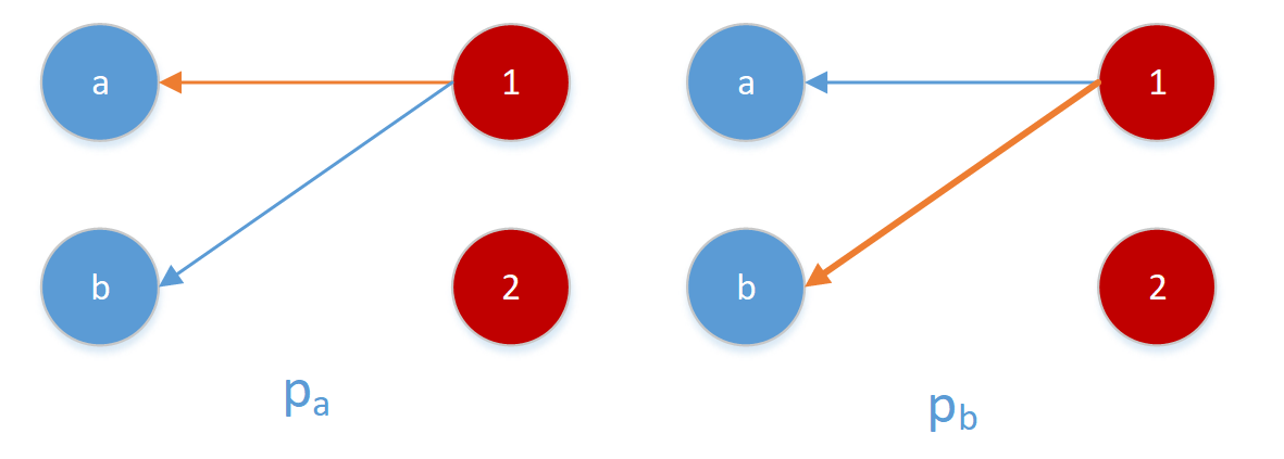
Knowing that with p_a the left scenario will happen in advance, the adversary needs to choose which edge can harm the performance of the algorithm the most. If the adversary chooses (2-a) edge in advance, then the expected matching becomes $ p_a + 2 * (1-p_a) $ and if he uses (2-b) then the expected matching becomes $ p_a * 2 (1-p_a) $. So he will choose the maximum. $ max⁡(p_a+(1-p_a ) * 2 ,p_a * 2+(1-p_a)) $. Therefore, the best action for the algorithm is to minimize it by trying to balance these two terms. Hence $ p_a=1/2 $.

In the example above, we would expect the best algorithm to choose each of two neighbors with the same probability to not allow adversarial to take any advantageous. What we would expect from the algorithm in the general setting?

The algorithm should match in a way that the adversary cannot predict its behavior. So in each step, the probability that the algorithm matches any of its free neighbors should be the same, otherwise, the adversary might take advantage of this difference. How we can do this?
One way to make such an algorithm is simply choosing a random permutation (a ranking) of left vertices at the beginning and upon the arrival of each right node, match it to its lowest rank free neighbor. This way guarantees that, in each step, knowing what happened in the past, the probability of matching to any of the free neighbors will be the same. This statement is true because knowing the matched neighbors gives us no information about the rank of other non-matched neighbors. (Intuitively this means that each right vertex spreads fractionally and evenly one unit of matching to its free neighbors. And this might be the most conservative greedy action.)

It seems that this algorithm works well! Now we want to find the worst-case scenario. We want to make sure that our algorithm is a good one. This might be the hardest part because we need to put ourselves in the shoes of the adversary. Adversary’s job is not an easy task. Knowing the algorithm, he wants to find the worst case!

Randomized Primal-Dual Analysis

One of the easiest ways to find a bound on the worst-case scenario on the expected competitive ratio, $ \frac{E(ALG)}{Offline} $ is to use the primal-dual analysis explained in Devanur et al. (SODA13). The great thing about the primal-dual analysis is that it decouples out the complexity of thinking about all possible combinations of edges that might be in the worst-case setting. Instead, it encapsulates all the information needed for analyzing the worst case in the dual variables.

Primal Problem

\(max \sum\nolimits_{e \in E} x_e\)
subject to
\(\sum\nolimits_{e \in \delta(v)} x_e \leq 1\) for all $ v \in V $
\(x_e \geq 0\) for all $ e \in E $

Dual Problem

\(min \sum\nolimits_{v \in V} p_v\)
subject to
\(p_v + p_w \geq 1\) for all $(v,w) \in E $
\(p_v \geq 0\) for all $v \in V$

The idea of this type of analysis is as follow:
We want to show that for any possible bipartite graph $G(V={L \cup R},E)$, the ratio between expected performance of algorithm and offline matching is bigger than some number F. We also know that any feasible solution of dual problem gives an upper bound for the primal problem. Therefore, we will show that any possible matching outcome corresponds to a vector $ q \subseteq \mathbb{R}^{|V|}$ so that $ ||q||_1 $ is the number of matching. At the same time, we will show that $\frac{1}{F} q $ is a random variable whose expeteced value is also a feasible dual solution. Therefore, $\frac{1}{F} \mathbb{E} ||q||_1 \geq \text{offline match}$ (by weak duality). To show this, it is enough to show the feasiblity for each edge separately. (i.e. the expected value of $q_v/F + q_w/F$ is bigger than 1.) Since all possible permutations have the same probability, we can calculate this expectation easily. (Please note that, we could not expect the random vector $q/F$ to be feasible all the time with F bigger than half, otherwise, we would be able to beat the half without any randomization.)
Karp, Vazirani, Vazirani also showed that this ratio is the best achievable ratio.

Stochastic Adversary

To make our problem close to the real world problem, it is useful to add more distributional assumption about the possible graph instances. This way, the adversary will be restricted to act according to a specific class of distribution hence we can hope for smarter algorithms with better bounds.
One way is to add assumption about preferences of advertisers. The advertisers are generally interested in some type of customers and these preferences can be a given information to the algorithm. The algorithm can also know the frequency of arrival of each type of customers. The algorithm then uses this information for the matching. For instance, Feldman et al. (FOCS09) beat 1-1/e in this setting.

There are different ways to add more realistic assumption about the real world problem and different ways to define the online version of matching. The problem that I worked on, is online stochatic matching which has a different setting.

.