Text Classification
Date:
In this project, we used 3 different metrics (Information Gain, Mutual Information, Chi Squared) to find important words and then we used them for the classification task. We compared the result at the end.
This project has two parts. In the first part, we find features (words which are highly related to the topics). In the second part, we classify documents, using different feature sets and evaluate the results.
Part 1
Each document can be represented by the set of words that appear in it.
But some words are more important and has more effect for determination of the context of the document.
So we want to represent a document by a set of important words. In this part, we are going to find a set of 100 words that are more infomative for document classification.
Data Set
The dataset for this task is “همشهری” (Hamshahri) that contains 8600 persian documents.
Preproceesing
We did some preprocessing for building our data structures for processing.
We read each document and added its words to our vocabulary set and also a set for that document.
We then used this set to create a vocab_index dictionary for assigning an index for each word that appears in our dataset.
Our dataset consists of 5 different classes.
class_name
['ورزش', 'اقتصاد', 'ادب و هنر', 'اجتماعی', 'سیاسی']
There is some statistcs information about out dataset.
print("vocab size:", len(vocab))
print ("number of terms (all tokens):", number_of_terms)
print ("number of docs:", number_of_docs)
print ("number of classes:", cls_index)
vocab size: 65880
number of terms (all tokens): 3506727
number of docs: 8600
number of classes: 5
The probability of each classes are stored in the table below.
tmp_view = pd.DataFrame(probability_of_classess)
tmp_view
| 0 | |
|---|---|
| 0 | 0.232558 |
| 1 | 0.255814 |
| 2 | 0.058140 |
| 3 | 0.209302 |
| 4 | 0.244186 |
# Calculation of our metrics for each words in Vocabulary We are going to find 100 words that are good indicator of classes.
We want to use 3 different type of metrics
- Information Gain
- Mutual Information
- $\chi$ square
Information Gain
We used these metric. And the top 10 words with highest information gain can be seen in the table below.
preview.head(10)
| information_gain | word | |
|---|---|---|
| 0 | 0.612973 | ورزشی |
| 1 | 0.516330 | تیم |
| 2 | 0.297086 | اجتماعی |
| 3 | 0.293313 | سیاسی |
| 4 | 0.283891 | فوتبال |
| 5 | 0.267878 | اقتصادی |
| 6 | 0.225276 | بازی |
| 7 | 0.223381 | جام |
| 8 | 0.197755 | قهرمانی |
| 9 | 0.177807 | اسلامی |
If you think about the meaning of these words you can agree that since they a have high information gain they can be really good identifiers for categorizing a doc.
In the table below, you can see 5 worst words.
preview.tail(5)
| information_gain | word | |
|---|---|---|
| 65875 | 0.000042 | تبهکاران |
| 65876 | 0.000042 | پذیرفتم |
| 65877 | 0.000041 | توقف |
| 65878 | 0.000031 | سلمان |
| 65879 | 0.000027 | چهارمحال |
Mutual Information
There is two formula for this metrics.
Another one is introduced in Website: https://nlp.stanford.edu/IR-book/html/htmledition/mutual-information-1.html
We used both of them and then choose the better set.
Let's see the result of each of those different formulae for this metric.
First Model:
Calculating with formula in the Slides:
\[MI(w, c_i) = \log{\frac{p(w, c_i)}{p(w)*p(c_i)}}\]The result is
preview.head(10)
| mutual information(MI) | main class MI | main_class | word | |
|---|---|---|---|---|
| 0 | 0.524418 | 1.782409 | ادب و هنر | مایکروسافت |
| 1 | 0.524418 | 1.782409 | ادب و هنر | باغات |
| 2 | 0.524418 | 1.782409 | ادب و هنر | نباریدن |
| 3 | 0.524191 | 1.703799 | اقتصاد | آلیاژی |
| 4 | 0.524191 | 1.703799 | اقتصاد | دادمان |
| 5 | 0.524191 | 1.703799 | اقتصاد | فرازها |
| 6 | 0.524191 | 1.703799 | اقتصاد | سیاتل |
| 7 | 0.521680 | 1.782409 | ادب و هنر | سخیف |
| 8 | 0.521680 | 1.782409 | ادب و هنر | کارناوال |
| 9 | 0.521680 | 1.782409 | ادب و هنر | تحتانی |
But there is a __problem__ here
The words in the table above, are infrequent words and because of that, they give use high information when they appear in a doc, but the probability of appearing such a word in any document is really small. So, in general, these words are not good identifiers.
You can see number of occurance of some of these words in each classes:
word_occurance_frequency_vs_class[word_index['نباریدن']], word_occurance_frequency_vs_class[word_index['مایکروسافت']], word_occurance_frequency_vs_class[word_index['آلیاژی']]
(array([0, 4, 1, 0, 0]), array([0, 4, 1, 0, 0]), array([0, 5, 1, 0, 0]))
Second Model
Now we want to calculate it with formula in this link.
The formula is:
\[MI(w, c_i) = \sum_{i,j \subset \{ 0 , 1 \}} {p(w=i, c_i=j)} * \log{\frac{p(w=i, c_i=j)}{p(w=i)*p(c_i=j)}}\]| mutual information(MI) | main class MI | main_class | word | |
|---|---|---|---|---|
| 0 | 0.202674 | 0.606665 | ورزش | ورزشی |
| 1 | 0.173929 | 0.512590 | ورزش | تیم |
| 2 | 0.099833 | 0.279402 | ورزش | فوتبال |
| 3 | 0.094818 | 0.258578 | سیاسی | سیاسی |
| 4 | 0.088517 | 0.232945 | اقتصاد | اقتصادی |
| 5 | 0.085858 | 0.265246 | اجتماعی | اجتماعی |
| 6 | 0.076582 | 0.209092 | ورزش | بازی |
| 7 | 0.076098 | 0.217883 | ورزش | جام |
| 8 | 0.070387 | 0.195426 | ورزش | قهرمانی |
| 9 | 0.056253 | 0.155666 | ورزش | بازیکن |
These words are better
They are not rare
You can see the frequency of some of these words in each classes:
print (list(reversed(class_name)))
word_occurance_frequency_vs_class[word_index['ورزشی']], word_occurance_frequency_vs_class[word_index['سیاسی']],  word_occurance_frequency_vs_class[word_index['پیروزی']],
['سیاسی', 'اجتماعی', 'ادب و هنر', 'اقتصاد', 'ورزش']


(array([1866,    9,    8,   66,   16]),
 array([  35,  300,   71,  372, 1602]),
 array([497,  44,  24,  60, 191]))
$ \chi$ Squared
Another Metric is $ \chi$ Squared.
Now we are goind to see the result of using $\chi$ squared as a mesure of importance.
| chi squared | main class chi | main_class | word | |
|---|---|---|---|---|
| 0 | 2234.591600 | 7376.515420 | ورزش | ورزشی |
| 1 | 2028.186959 | 6701.136193 | ورزش | تیم |
| 2 | 1302.947803 | 4296.622009 | ورزش | فوتبال |
| 3 | 1050.289281 | 3459.737651 | ورزش | جام |
| 4 | 1043.478941 | 3138.957039 | سیاسی | سیاسی |
| 5 | 1029.481451 | 3055.759330 | اقتصاد | اقتصادی |
| 6 | 1027.311167 | 3254.137538 | ورزش | بازی |
| 7 | 967.923254 | 3299.353018 | اجتماعی | اجتماعی |
| 8 | 961.078769 | 3169.912598 | ورزش | قهرمانی |
| 9 | 772.041205 | 2558.041173 | ورزش | بازیکن |
Result Comparison
We can compare our three set of words here.
In the table below, you can see top 20 words for each metrics.
For mutual information, there are two sets because we used two different formula.
| information gain1 | chi squared1 | mutual information_model_2 | mutual information_model_1 | |
|---|---|---|---|---|
| 0 | ورزشی | ورزشی | ورزشی | مایکروسافت |
| 1 | تیم | تیم | تیم | باغات |
| 2 | اجتماعی | فوتبال | فوتبال | نباریدن |
| 3 | سیاسی | جام | سیاسی | آلیاژی |
| 4 | فوتبال | سیاسی | اقتصادی | دادمان |
| 5 | اقتصادی | اقتصادی | اجتماعی | فرازها |
| 6 | بازی | بازی | بازی | سیاتل |
| 7 | جام | اجتماعی | جام | سخیف |
| 8 | قهرمانی | قهرمانی | قهرمانی | کارناوال |
| 9 | اسلامی | بازیکن | بازیکن | تحتانی |
| 10 | بازیکن | بازیکنان | اسلامی | معراج |
| 11 | مجلس | فدراسیون | بازیکنان | خلافت |
| 12 | بازیکنان | مسابقات | فدراسیون | نجیب |
| 13 | فدراسیون | دلار | مسابقات | زبون |
| 14 | مسابقات | قیمت | دلار | صحیفه |
| 15 | شورای | مسابقه | مسابقه | مشمئزکننده |
| 16 | مسابقه | آسیا | مجلس | ارتجاع |
| 17 | دلار | گذاری | قیمت | ذبیح |
| 18 | آسیا | صنایع | شورای | وصنایع |
| 19 | مردم | سرمایه | گذاری | توپخانه |
Output File
The output files are stored in CSV format files.
These files contain 100 most important words for each metrics.
Conclusion of Part 1
When you look at the last table you can see first three columns are similar to each other and have nearly same words but last columns’ (mutual information with formula 1) words are different from other columns
We can conclude that the Formula 1 has different behavior and probably is not efficient. So it is better to use formula 2 for calculating Mutual Information
For more accurate comparisons on which of these three metrics are better, we can test it.
In part 2 we are going to test which metric is better, with a classification task.
Part 2
In Part 1 we tried to find good features to vectorize documents. We used three metrics and extracted three set of 100 words.
Each document can be represented by the set of words that appear in the document.
In this part we want to use these sets of features to classify documents with SVM.
Evaluation
For evaluating our classification we used k-fold cross-validation with k=5.
We reported our average of these 5 confusion matrices.
## Vectorizing Documents We wanted to vectorize our documents. We did this with 4 different methods:
1) Using 1000 most frequent words as features set
2) Using Information Gain features
3) Using Mutual Information features
4) Using $\chi$ square features
Storing word frequencies
We need to store word frequency in each document for the processing
1) Using 1000 most frequent words as feature set
There is an ambiguity in defining the meaning of frequent.
- First meaning: A word is frequent if in lots of document there is at least one occurrence of this word.
- Second meaning: A word is frequent if the sum of the number of occurrence of this word in all documents is high. (Maybe in one document there are lots of occurrences but in another document, there is no occurrence.)
In this code, we chose the first meaning.
| 0 | 1 | |
|---|---|---|
| 0 | 8415 | و |
| 1 | 8352 | در |
| 2 | 8241 | به |
| 3 | 7956 | از |
| 4 | 7838 | این |
| 5 | 7382 | با |
| 6 | 7240 | که |
| 7 | 6923 | را |
| 8 | 6912 | است |
| 9 | 6859 | می |
The above words are 10 most frequent words in our dataset. And all of them are stop words.
Making Vector X
We want to make the vector for each document and then use this vectors for classification.
We used our 1000 words for vectorizing.
Using SVM for classification
We used svm classifier for our classification.
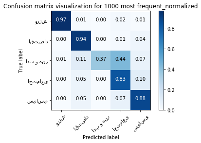
Confusion Matrix for 1000 most frequent
print ("accuracy:", first_method_accuracy,'\n')
print ("confusion matrix:\n")
first_method_cm = confusion_matrix_avg
pd.DataFrame(first_method_cm)
accuracy: 0.8787209302325582

confusion matrix:
| 0 | 1 | 2 | 3 | 4 | |
|---|---|---|---|---|---|
| 0 | 389.0 | 2.2 | 0.0 | 6.4 | 2.4 |
| 1 | 0.2 | 414.2 | 0.2 | 6.4 | 19.0 |
| 2 | 1.2 | 10.8 | 37.2 | 44.2 | 6.6 |
| 3 | 1.6 | 18.4 | 1.6 | 300.6 | 37.8 |
| 4 | 1.0 | 19.2 | 0.0 | 29.4 | 370.4 |
2) Using 100-dimensional vector with Information Gain
| information_gain | word | |
|---|---|---|
| 0 | 0.612973 | ورزشی |
| 1 | 0.516330 | تیم |
| 2 | 0.297086 | اجتماعی |
| 3 | 0.293313 | سیاسی |
| 4 | 0.283891 | فوتبال |
| 5 | 0.267878 | اقتصادی |
| 6 | 0.225276 | بازی |
| 7 | 0.223381 | جام |
| 8 | 0.197755 | قهرمانی |
| 9 | 0.177807 | اسلامی |
Making Vector X
We want to make vector for each document and then use this vectors for classification
Using SVM for classification
print ("accuracy:", second_method_accuracy,'\n')
print ("confusion matrix:\n")
second_method_cm = confusion_matrix_avg
pd.DataFrame(second_method_cm)
accuracy: 0.806279069767442

confusion matrix:
| 0 | 1 | 2 | 3 | 4 | |
|---|---|---|---|---|---|
| 0 | 376.0 | 7.6 | 0.2 | 11.4 | 4.8 |
| 1 | 1.4 | 382.6 | 0.2 | 22.0 | 33.8 |
| 2 | 4.0 | 24.0 | 7.2 | 55.0 | 9.8 |
| 3 | 2.4 | 30.8 | 1.0 | 268.8 | 57.0 |
| 4 | 2.4 | 31.6 | 0.2 | 33.6 | 352.2 |
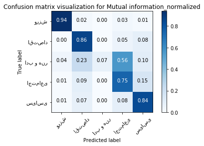
3) Using 100-dimensional vector with Mutal Information
We used the better formula for selecting 100 words.
features.head(10)
| mutual information | main class score | main class | word | |
|---|---|---|---|---|
| 0 | 0.202674 | 0.606665 | ورزش | ورزشی |
| 1 | 0.173929 | 0.512590 | ورزش | تیم |
| 2 | 0.099833 | 0.279402 | ورزش | فوتبال |
| 3 | 0.094818 | 0.258578 | سیاسی | سیاسی |
| 4 | 0.088517 | 0.232945 | اقتصاد | اقتصادی |
| 5 | 0.085858 | 0.265246 | اجتماعی | اجتماعی |
| 6 | 0.076582 | 0.209092 | ورزش | بازی |
| 7 | 0.076098 | 0.217883 | ورزش | جام |
| 8 | 0.070387 | 0.195426 | ورزش | قهرمانی |
| 9 | 0.056253 | 0.155666 | ورزش | بازیکن |
Making Vector X
We want to make vector for each document and then use this vectors for classification
Using SVM for classification
print ("accuracy:", third_method_accuracy,'\n')
print ("confusion matrix:\n")
third_method_cm = confusion_matrix_avg
pd.DataFrame(third_method_cm)
accuracy: 0.804186046511628

confusion matrix:
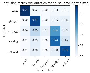
| 0 | 1 | 2 | 3 | 4 | |
|---|---|---|---|---|---|
| 0 | 375.2 | 8.2 | 0.0 | 11.4 | 5.2 |
| 1 | 1.4 | 379.8 | 0.2 | 22.6 | 36.0 |
| 2 | 3.8 | 23.0 | 7.0 | 56.4 | 9.8 |
| 3 | 2.0 | 31.4 | 1.0 | 270.0 | 55.6 |
| 4 | 2.4 | 31.2 | 0.2 | 35.0 | 351.2 |
4) Using 100-dimensional vector with $\chi$ Squared
features.head(10)
| chi squared | main class score | main class | word | |
|---|---|---|---|---|
| 0 | 2234.591600 | 7376.515420 | ورزش | ورزشی |
| 1 | 2028.186959 | 6701.136193 | ورزش | تیم |
| 2 | 1302.947803 | 4296.622009 | ورزش | فوتبال |
| 3 | 1050.289281 | 3459.737651 | ورزش | جام |
| 4 | 1043.478941 | 3138.957039 | سیاسی | سیاسی |
| 5 | 1029.481451 | 3055.759330 | اقتصاد | اقتصادی |
| 6 | 1027.311167 | 3254.137538 | ورزش | بازی |
| 7 | 967.923254 | 3299.353018 | اجتماعی | اجتماعی |
| 8 | 961.078769 | 3169.912598 | ورزش | قهرمانی |
| 9 | 772.041205 | 2558.041173 | ورزش | بازیکن |
Making Vector X
We want to make vector for each document and then use this vectors for classification
Using SVM for classification
print ("accuracy:", forth_method_accuracy,'\n')
print ("confusion matrix:\n")
forth_method_cm = confusion_matrix_avg
pd.DataFrame(forth_method_cm)
accuracy: 0.8025581395348838

confusion matrix:
| 0 | 1 | 2 | 3 | 4 | |
|---|---|---|---|---|---|
| 0 | 375.2 | 8.2 | 0.0 | 11.4 | 5.2 |
| 1 | 1.4 | 380.8 | 0.2 | 22.2 | 35.4 |
| 2 | 3.8 | 25.0 | 6.6 | 55.6 | 9.0 |
| 3 | 2.4 | 31.2 | 0.8 | 267.2 | 58.4 |
| 4 | 2.4 | 31.8 | 0.2 | 35.0 | 350.6 |
Comparision
We compare our result with these 4 methods with confusion matrix and accuracy
The result is as follow
preview = pd.DataFrame({'1000words': [first_method_accuracy],
                        'InfoGain': [second_method_accuracy],
                        'mutual info': [third_method_accuracy],
                        "chi squared": [forth_method_accuracy]})
print ("accuracy:")
preview
accuracy:
| 1000words | InfoGain | chi squared | mutual info | |
|---|---|---|---|---|
| 0 | 0.878721 | 0.806279 | 0.802558 | 0.804186 |
preview = pd.concat([pd.DataFrame(first_method_confusion_matrix),
                     pd.DataFrame(second_method_confusion_matrix),
                     pd.DataFrame(third_method_confusion_matrix),
                     pd.DataFrame(forth_method_confusion_matrix)], axis=1)
print ("confusion matrix:")
print ("\t1000 words\t\t\t IG \t\t \t MI \t\t   chi squared")
preview
confusion matrix:
	1000 words			 IG 		 	 MI 		   chi squared
| 0 | 1 | 2 | 3 | 4 | 0 | 1 | 2 | 3 | 4 | 0 | 1 | 2 | 3 | 4 | 0 | 1 | 2 | 3 | 4 | |
|---|---|---|---|---|---|---|---|---|---|---|---|---|---|---|---|---|---|---|---|---|
| 0 | 389.0 | 2.2 | 0.0 | 6.4 | 2.4 | 376.0 | 7.6 | 0.2 | 11.4 | 4.8 | 375.2 | 8.2 | 0.0 | 11.4 | 5.2 | 375.2 | 8.2 | 0.0 | 11.4 | 5.2 |
| 1 | 0.2 | 414.2 | 0.2 | 6.4 | 19.0 | 1.4 | 382.6 | 0.2 | 22.0 | 33.8 | 1.4 | 379.8 | 0.2 | 22.6 | 36.0 | 1.4 | 380.8 | 0.2 | 22.2 | 35.4 |
| 2 | 1.2 | 10.8 | 37.2 | 44.2 | 6.6 | 4.0 | 24.0 | 7.2 | 55.0 | 9.8 | 3.8 | 23.0 | 7.0 | 56.4 | 9.8 | 3.8 | 25.0 | 6.6 | 55.6 | 9.0 |
| 3 | 1.6 | 18.4 | 1.6 | 300.6 | 37.8 | 2.4 | 30.8 | 1.0 | 268.8 | 57.0 | 2.0 | 31.4 | 1.0 | 270.0 | 55.6 | 2.4 | 31.2 | 0.8 | 267.2 | 58.4 |
| 4 | 1.0 | 19.2 | 0.0 | 29.4 | 370.4 | 2.4 | 31.6 | 0.2 | 33.6 | 352.2 | 2.4 | 31.2 | 0.2 | 35.0 | 351.2 | 2.4 | 31.8 | 0.2 | 35.0 | 350.6 |
Visualization
We are going to show each one in separated tables:
plt.figure()
plot_confusion_matrix(first_method_cm, classes=class_name,
                      title='Confusion matrix visualization for 1000 most frequent_normalized', normalize=True);
plt.show()
plt.figure()
plot_confusion_matrix(second_method_cm, classes=class_name,
                      title='Confusion matrix visualization for Information gain_normalized', normalize=True);
plt.show()
plt.figure()
plot_confusion_matrix(third_method_cm, classes=class_name,
                      title='Confusion matrix visualization for Mutual information_normalized', normalize=True);
plt.show()
plt.figure()
plot_confusion_matrix(forth_method_cm, classes=class_name,
                      title='Confusion matrix visualization for chi squared_normalized', normalize=True);
plt.show()
Now we want to test the result for most 100 frequent word vector
print ("accuracy:", first_method_accuracy_100,'\n')
print ("confusion matrix:\n")
first_method_cm_100 = confusion_matrix_avg
pd.DataFrame(first_method_cm_100)
accuracy: 0.803953488372093

confusion matrix:
| 0 | 1 | 2 | 3 | 4 | |
|---|---|---|---|---|---|
| 0 | 375.6 | 8.2 | 0.0 | 11.4 | 4.8 |
| 1 | 1.4 | 382.4 | 0.4 | 22.0 | 33.8 |
| 2 | 3.2 | 24.8 | 7.2 | 55.2 | 9.6 |
| 3 | 1.8 | 30.8 | 1.0 | 267.4 | 59.0 |
| 4 | 2.4 | 32.6 | 0.2 | 34.6 | 350.2 |
plt.figure()
plot_confusion_matrix(first_method_confusion_matrix_100, classes=class_name,
                      title='Confusion matrix visualization for 100 most frequent_normalized', normalize=True);
plt.show()

Conclusion
We know that 1000 words are not best words because these words include stop words that they are not informative. But because they are 1000 words rather than 100 words, the result is going to be better.
We test a set of 100 most frequent words. The result was acc = 0.8049 which is similar to other three methods. We also show the confusion matrix for 100 most frequent in the last table above. And you can see this table is also similar to other three ones
So we can guess that there is no significant difference between choosing these metrics for selecting words in document classification task.
And we also know that Information Gain doesn’t store every class information gains (We only stored one number Information Gain for every word). But we can consider each class information gain if we split the Sigma over classes in information gain formula.(And consider the meaning of Entropy for each class). So it has the same functionality as other metrics.
We guess that if the dimension of our vector increase we probably are going to get more accuracy.
And also maybe if we use different features depending on the sequence of words that appear each document, we can get more accuracy.