In 1990 Karp, and Vazirani and Vazirani published a paper called an Optimal Algorithm for on-line bipartite matching which introduces the ranking algorithm. They showed that their algorithm achieves (1-1/e) competitive ratio (comparing to offline version,) and no other algorithm can beat this ratio. This paper was a starting point for lots of future works. So it is useful to take a close look at their algorithm and ways to analyze it.

What is on-line Bipartite Matching?

There are different ways to introduce an on-line version of Bipartite matching. One of them is motivated by Internet advertising display applications. In this setting, users search for a keyword and the algorithm wants to match users to some relevant advertisers. The advertisers (left vertices) are known in advance and they just prefer to match to relevant users. Users (right vertices) arrive online as they search in the search engine. Upon their arrival, the algorithm should match one of the interested advertisers to the user (i.e. Display the corresponding ad) or ignore the users. In the original setting of Karp, Vazirani, Vazirani there was no priory assumption about the type of users and advertisers can have arbitrary any function for determining whether a user is relevant to them or not.

So here the challenge is that we need to choose a permanent action (matching) before knowing all information about the problem (just like any online algorithm problem). If we were allowed to change our past decisions, then on the arrival of each right node, we would be able to match optimally whether by matching it to a free neighbor or by just a chain of swapping of matched nodes. But now upon the arrival of each node, we need to match it permanently or leave it free.

A simple algorithm
Upon the arrival of each vertex, match it to its lowest index free neighbors if it has any.

This algorithm and any other algorithm that matches whenever it can (a maximal match), is always at least as good as half of the optimum offline solution (maximum-mal match). Because this statement is true for any two maximal matches. So we can simply achieve a 0.5 competitive ratio, but can we do better?

The adversary

To determine whether we can perform better than half, we need to think about the worst-case scenario for each algorithm that we want to analyze. It is useful to think about the worst-case as an adversary trying to bring us the worst-case instance. Here, it is crucial to define the strength and limitations of the adversary. We define three possible adversaries:

Strong adversary

This type of adversary is a bit stronger than usual adversary types but let’s define it for future discussion! This type of adversary needs to choose the number of left vertices at the beginning. Then the game starts. In each step, the adversary might add a new right node and identify its left neighbors or terminates the game otherwise. Upon the arrival of each node, the algorithm might match it or not. But based on her action, the adversary will do the next action. The adversary might end the game after any number of steps. Competing against this type of adversary to get a better competitive ratio than half is a hopeless job. Because this type of adversary is really strong as he can identify the neighborhood of each right node after observing the algorithm’s actions. For instance, the adversary can do the following strategy to get the half competitive ratio:
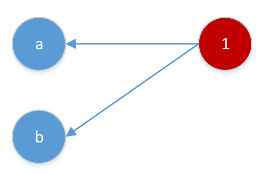
He chooses the number of left vertices to be 2 at the beginning and in the first step, he identifies the neighbors of the first right node as follows:

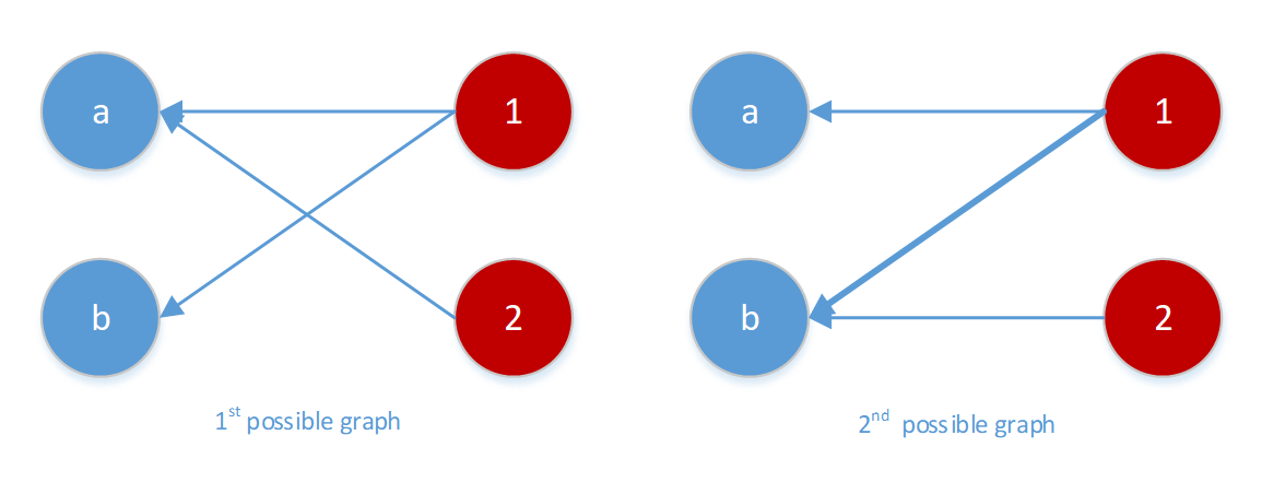
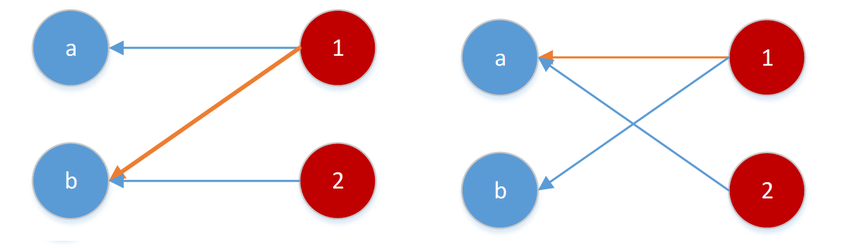
Based on the action done by the algorithm (which is shown by the orange arrow), the adversary will show one of the following neighbors for the next vertex.

In any of these two scenarios, the second node cannot get matched. The adversary will terminate the game in this step. We left with one match while the off-line version for both graphs matches both right vertices. So the worst case competitive ratio is exactly half and not more. Therefore, to beat the half, we need to restrict the strength of the adversary.

Normal Adversary

This type of adversary is just the usual adversary. This adversary knows the algorithm that we are going to use at the beginning, he should identify the entire bipartite graph before the algorithm makes any decision. Here, if the algorithm is a deterministic one, the normal adversary is as strong as the stronger type of adversary as he can predict the actions done by algorithm precisely at the beginning and construct the bipartite graph accordingly. Therefore, we need to add randomness to our algorithm to have any chance of beating the half! We want to make an unpredictable algorithm to not allowing the normal adversary to act as a strong adversary.

Let’s try to find a good algorithm!

Ok. Let’s think about what we would expect from our algorithm in instances that have two left vertices and then try to generalize our strategy for any possible bipartite graph.
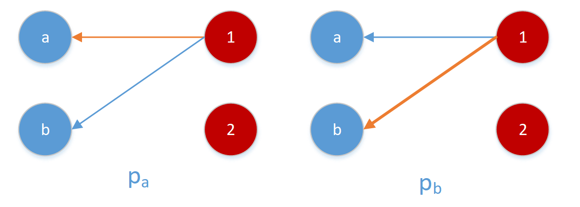
In the beginning, our algorithm sees the first vertex (call it “1”) and its neighbors that adversary designed for us. If “1” has a single neighbor, there is no harm to match it in any possible scenario so we expect our algorithm to match it. But if “1” has two neighbors (a and b), our algorithm should identify that with what probability we will match it to “a” ($p_a$ ) and or to “b ($p_b$ ). (There is no point in not matching it, so this action has zero probability and $p_a+p_b=1$.) To find the best possible $ p_a,p_b $, we need to understand the behavior of adversary for any fixed $ p_a,p_b $. So let’s put ourselves to the adversary’s shoes.

Knowing that with p_a the left scenario will happen in advance, the adversary needs to choose which edge can harm the performance of the algorithm the most. If the adversary chooses (2-a) edge in advance, then the expected matching becomes $ p_a + 2 * (1-p_a) $ and if he uses (2-b) then the expected matching becomes $ p_a * 2 (1-p_a) $. So he will choose the maximum. $ max⁡(p_a+(1-p_a ) * 2 ,p_a * 2+(1-p_a)) $. Therefore, the best action for the algorithm is to minimize it by trying to balance these two terms. Hence $ p_a=1/2 $.

In the example above, we would expect the best algorithm to choose each of two neighbors with the same probability to not allow adversarial to take any advantageous. What we would expect from the algorithm in the general setting?

The algorithm should match in a way that the adversary cannot predict its behavior. So in each step, the probability that the algorithm matches any of its free neighbors should be the same, otherwise, the adversary might take advantage of this difference. How we can do this?
One way to make such an algorithm is simply choosing a random permutation (a ranking) of left vertices at the beginning and upon the arrival of each right node, match it to its lowest rank free neighbor. This way guarantees that, in each step, knowing what happened in the past, the probability of matching to any of the free neighbors will be the same. This statement is true because knowing the matched neighbors gives us no information about the rank of other non-matched neighbors. (Intuitively this means that each right vertex spreads fractionally and evenly one unit of matching to its free neighbors. And this might be the most conservative greedy action.)

It seems that this algorithm works well! Now we want to find the worst-case scenario. We want to make sure that our algorithm is a good one. This might be the hardest part because we need to put ourselves in the shoes of the adversary. Adversary’s job is not an easy task. Knowing the algorithm, he wants to find the worst case!

Randomized Primal-Dual Analysis

One of the easiest ways to find a bound on the worst-case scenario on the expected competitive ratio, $ \frac{E(ALG)}{Offline} $ is to use the primal-dual analysis explained in Devanur et al. (SODA13). The great thing about the primal-dual analysis is that it decouples out the complexity of thinking about all possible combinations of edges that might be in the worst-case setting. Instead, it encapsulates all the information needed for analyzing the worst case in the dual variables.

Primal Problem

\(max \sum\nolimits_{e \in E} x_e\)
subject to
\(\sum\nolimits_{e \in \delta(v)} x_e \leq 1\) for all $ v \in V $
\(x_e \geq 0\) for all $ e \in E $

Dual Problem

\(min \sum\nolimits_{v \in V} p_v\)
subject to
\(p_v + p_w \geq 1\) for all $(v,w) \in E $
\(p_v \geq 0\) for all $v \in V$

The idea of this type of analysis is as follow:
We want to show that for any possible bipartite graph $G(V={L \cup R},E)$, the ratio between expected performance of algorithm and offline matching is bigger than some number F. We also know that any feasible solution of dual problem gives an upper bound for the primal problem. Therefore, we will show that any possible matching outcome corresponds to a vector $ q \subseteq \mathbb{R}^{|V|}$ so that $ ||q||_1 $ is the number of matching. At the same time, we will show that $\frac{1}{F} q $ is a random variable whose expeteced value is also a feasible dual solution. Therefore, $\frac{1}{F} \mathbb{E} ||q||_1 \geq \text{offline match}$ (by weak duality). To show this, it is enough to show the feasiblity for each edge separately. (i.e. the expected value of $q_v/F + q_w/F$ is bigger than 1.) Since all possible permutations have the same probability, we can calculate this expectation easily. (Please note that, we could not expect the random vector $q/F$ to be feasible all the time with F bigger than half, otherwise, we would be able to beat the half without any randomization.)
Karp, Vazirani, Vazirani also showed that this ratio is the best achievable ratio.

Stochastic Adversary

To make our problem close to the real world problem, it is useful to add more distributional assumption about the possible graph instances. This way, the adversary will be restricted to act according to a specific class of distribution hence we can hope for smarter algorithms with better bounds.
One way is to add assumption about preferences of advertisers. The advertisers are generally interested in some type of customers and these preferences can be a given information to the algorithm. The algorithm can also know the frequency of arrival of each type of customers. The algorithm then uses this information for the matching. For instance, Feldman et al. (FOCS09) beat 1-1/e in this setting.

There are different ways to add more realistic assumption about the real world problem and different ways to define the online version of matching. The problem that I worked on, is online stochatic matching which has a different setting.

.

Let’s talk about the competition between navigation apps first:

Of course, all of the navigator applications try to increase their customers by providing better features. One of the most important features is the ability to find the fastest route for each customer. So the applications are designed in a way that if there is a better shortcut, that shortcut will be get used for customers to tempt them to use the same application for the next time. (instead of any other competitor apps.)

In other words, because we only use the application that gives us the best route every time, all companies inevitably should try their best to give us the best route every time otherwise their product will not be used anymore!
As a result, after a while, aside from the specific application that each individual uses, each individual is trying to find the best route for himself. In the following, we will explain why this is a bad thing for society!

Let’s define Average Travel Time

In this setting, each person has an average travel time. (Since we don’t have any information about each individual, and because, roughly speaking, each region in the city is similar to other regions, we can assume that the situation for each individual is the same and symmetric, so this average time is the amount of time we need to put for each travel)
There is a question arising in this setting. Does using this app necessarily lead to our city having the lowest possible average travel time for each individual? Or we can do better?
Someone might think that if each individual tries to minimize his travel time in each travel, then he is using routes less than the time when he doesn’t. So on aggregate, this will be the best possible choice for each individual. But this is not necessarily true. (I know it might be a little confusing for the first time, but wait), I will explain it using a very famous example which is called Baraess Paradox.

Braess Paradox

(All of the images here are from Game Theory Alive book [1])
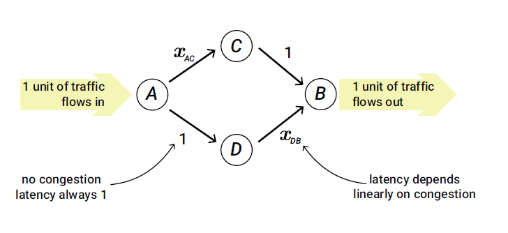
Suppose that we have 2 routes from A to B similar to the image below. Each edge in this graph has a latency function. We call it $l_e(x)$ where x is the number of cars in that edge.
Here, edges AD and CB have a constant latency function equals to one. $ l_{AD}(x)= l_{CB}(x)=1 $ (they represent streets which are sparse enough so that you can drive with the maximum speed of 30km/h without any trouble.)
Edges AC and DB have a latency proportional to the number of drivers that currently use that edge. $ l_{AC}(x) = l_{DB}(x) = x $ (You can assume that they are highways. On highways, you should keep your distance with the car in front of you in a way that if it immediately stopped, you would be able to react properly and stop your car. And the distance with that car is proportional to the number of cars using that route. i.e. If there are x cars on the highway, on average the car in front of you have d meter distance with you, on the other hand, if there are 2x cars, then on average the car in front of you have d/2 meters distance from you. so you need to decrease your speed from v to v/2 to keep your time distance with the car. as a result, the latency will increase from t to 2t.)

So in this setting, AC and DB are highways and we love to use them!

What will happen in this setting?

Ok so in that setting, what will happen? Suppose that $ 100.x $ percent of drivers like the top route and $ 100.(1-x) $ percent like the bottom route, then if $x\geq 0.5$ after a few days, those drivers who like the top route will notify that the bottom route is better, so they will lose their interest as time goes on. So we will see a decrease in the x population. If we plot the population for the top route each day, we will probably see a sequence converging to 0.5. If the $x\leq 0.5$ same things will happen to bottom route drivers.

So, after a few weeks, our expected latency would be:
1 + 0.5 for both top drivers and bottom drivers.

Adding a new road is not always good

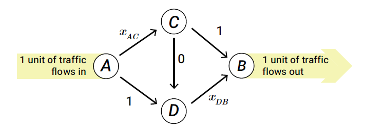
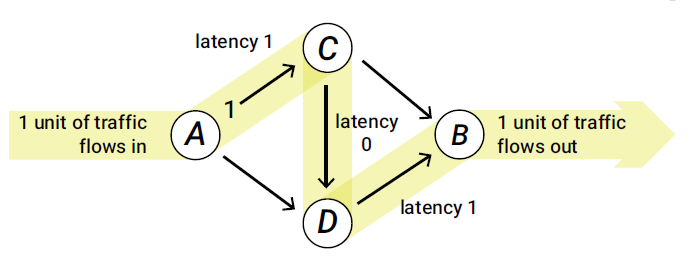
Now suppose we construct a shortcut from C to D with latency zero. Of course, adding a new line with no latency seems a good idea. People would love this. Because they can use the path A-C-D-B to use both of the highways. (Adding this shortcut is very similar to the situation in which people have access to a navigator app that knows local shortcuts from a highway to another. The app gives the best possible map for each individual that uses it)

Forget about the navigator app for a minute and suppose we are about to add our zero-latency shortcut.

What will happen?

The day after we construct this shortcut, the drivers of the top route will notice that A-C-D-B is a faster route. So they will become interested to change their path. They will use A-C-D-B and the DB highway will become more crowded. As a result, the bottom drivers (A-D-B) will try to use the top route (A-C-D). As they use it, they will notice that there is a new shortcut C-D. They will test it and realize that the best path is A-C-D-B. Finally, after a couple of weeks, all drivers will use A-C-D-B as their path. (In fact, this choice is a Nash equilibrium, meaning that after a day, nobody will have any regret about the path he chose, also note that there might be several Nash equilibria) It means that all of the drivers use two highways and as a result, we have two crowded highways that are like streets. As if there is no highway at all! That’s a tragedy! So adding a shortcut is not always a good idea.

Getting back to our navigation problem

Adding a shortcut is in some sense related to the use of this navigation applications. Sometimes they give us shortcuts to get away from congested traffic. But it doesn’t necessarily mean that what we are doing to the traffic will not make the condition even worse for ourselves. Of course, this example is a very simplified model that cannot capture all the properties of a city. These linear latency functions are good to model network connection and not necessarily the best choice for traffic in cities. But aside from these simplicity making assumptions, there is a fundamental flaw when all people try to only maximize their objective. This might be the case that the

The best for the group comes when everyone in the group does what’s best for himself AND the group.

In the game theory community, people try to find a bound on how bad it is for people to be selfish comparing to the best average result. They call this bound price of anarchy.

Price of Anarchy

In the above example, the price of anarchy is:
\(\text{price of anarchy} =: \frac {\text{average travel time in the worst Nash equilibrium}}{\text{average travel time in socially optimum outcome}}=\frac{2}{\frac{3}{2}}=\frac{4}{3}\)
So in this simple city, if no one uses the shortcut, we can have a better travel time. Ok. Let’s talk about a better model for traffic.

A better model

I saw this model from Section 8.4 Atomic Selfish Routing from [1] (which is a very great book, at least for me). This model is closer to our city.
I brought the definition of it from [1]:

Consider a road network G = (V;E) and a set of k drivers, with each driver i traveling from a starting node $s_i \in V$ to a destination $ t_i \in V$ . Associated with each edge $e \in E$ is a latency function$l_e(n) = a_e . n+b_e$ representing the cost of traversing edge e if n drivers use it. Driver i’s strategic decision is which path $P_i$ to choose from $s_i$ to $t_i$, and her objective is to choose a path with minimum latency.

To what extent we can hope for a better application

In the setting above, the price of anarchy is at most $ \frac{5}{2} $ . [1] Meaning that if we use the best social optimum paths, then the best thing we can hope for is to decrease our average latency by a factor of $ \frac{2}{5} $. If we assume that the model above is precise enough, then $ \frac{2}{5} $ is a bound on how bad the navigation apps affect the traffic compared to the best possible routing system.

Conclusion: What is the solution

What we know so far is that, there is a possibility that the price of anarchy in our city would be a big number. So we should verify it. (Perhaps, by collecting data and estimating the latency function and distribution of starting and ending locations and computing the estimated price of anarchy).
Suppose that it is verified that the price of anarchy in our city is a big number. In this case, the competition between different companies leads to this anarchy. Right now they do not have any incentive to give the social optimum route to each individual. So I can propose two naive ways-of courses there should be better solutions:

1) Restrict people to use a central app which gives us social optimum routes

2) Charge individuals for the route they choose based on the effect it has on the average traffic time.

Maybe we can find a good price function to incentivize people to use social optimum routes. Similar to the ideas related to Mechanism Design.

Resources:

1: Karlin, Anna R., and Yuval Peres. Game theory, alive. Vol. 101. American Mathematical Soc., 2017.

1. Since it works well on this dataset!
2. Because we want to give more penalty for bad predictions (in comparison with l1-norm)
3. Computing the derivation of MSE is simple (in comparison with l1-norm)
   

To be honest, The above reasons don’t convince me. In response to the first one we can say “ok it works well but there could be better choices” For the second and third reasons we can say: “there is another alternative for giving a penalty for a bad prediction (such as l4-norm) with easy computations.”

But fortunately, I found one reason (for a particular situation) in Wasserman’s “All of statistics” that makes me more relaxed! For other people not interested in the above reasons, I want to share this post to hopefully help them to be relaxed.
The book states that in linear regression with normal noise if we want to use Maximum Likelihood to learn parameter, it is the same as minimizing the MSE.
First, let’s define linear regression.

Definition of Random Variables

Suppose for each data, we have n-dimensional vector X and label Y. We assume that there is a linear relationship between X and Y. (ie. a.X+b=Y) thus we want to find the best candidate for (a,b). But the problem is that there are some unknown factors affecting the Y. We call them noise.
We can rewrite the equation:

$ Y(x) = a.x + b + Noise(x) $

There are different ways to find (a,b). In one way, we can think about (a,b) as random variables and we want to know which setting of (a,b) is the most likely one.
We also have to consider the noise as a random variable so we have to assign a distribution for the noise. We can imagine there are k independent unknown factors with different unknown distribution cumulatively affecting the Y. Because there are a lot of different small factors (k > 30), there is a more general theorem than Central Limit Theorem which states that:

No matter if series of factors have the same distribution or not, (when our factors are small enough and have some specific properties) the distribution of their sum converges in distribution to Normal distribution.

So when we have $ X = a $ ,our noise has the distribution like this:

$ PDF_{noise(X=a)}(x) = Normal(x, \mu_{X=a} , \sigma_{X=a} ) $

Here we suppose that in each point X=a, there are k independent factors. Now there is this question:
Do these k independent factors have different distributions in different Xs? Is the noise independent of the X or not?
I think we should take time and think about the noise being independent of the X and I’m going to present a reason for it here.

My Reason

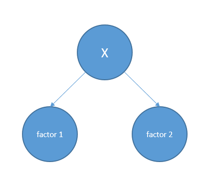
Suppose the knowing X=a is determiner of the distribution of each of the noises, so we have a probabilistic graphical model like this:

Having this model, factor1 and factor2 are dependent on each other. Because knowing factor1 can draw information about X and by having information about X, we would have information about factor2. But this contradicts with our independence assumption.

So we can rewrite it:

$ PDF_{noise}(x) = Normal(x, \mu , \sigma ) $

$ Y(x) = a.x + b + Noise $

Since there is a constant factor in the equation (b), without loss of generality, we can suppose the Normal Distribution has the mean equal to ZERO.

$ PDF_{noise}(x) = Normal(x, \mu=0 , \sigma ) $

Now, we want to find the most probable $ (a,b,\sigma)$ .

Now the probablity of Y is as follows:

$Y(x|a,b,\sigma) = a.X + b + Normal (0, \sigma^2) = Normal (a.X+b, \sigma^2 ) $

For finding the most probable configuration, we Use Maximum Likelihood Estimation.

Maximum Likelihood Estimation

Maximum likelihood estimation is a method used for finding the most likely parameters setting that can generate data samples. If we have m samples $(X_i, Y_i)$, and parameter $a, b $ then, we can calculate the probability of observation of data:

$ P (X,Y|a,b, \sigma) = \displaystyle\prod_{i=1}^{m} P(Y_i , X_i) = \displaystyle\prod_{i=1}^{m} P(X_i) P(Y_i | X_i) = \displaystyle\prod_{i=1}^{m} P(X_i) \displaystyle\prod_{i=1}^{m} P(Y_i | X_i) = $
$ \displaystyle\prod_{i=1}^{m} P(X_i) \displaystyle\prod_{i=1}^{m} Y(X_i|a,b,\sigma) = L1 * \displaystyle\prod_{i=1}^{m} Y(X_i|a,b,\sigma) $

We want to find $ (a,b,\sigma)$ that maximize the above likelihood. Since L1 is not a function of $ (a,b,\sigma)$ our parameters, we omit it and maximize the remaining part.

$ P (X,Y|a,b, \sigma) \propto \displaystyle\prod_{i=1}^{m} Y(X_i|a,b,\sigma)= \displaystyle\prod_{i=1}^{m} Normal (a.X_i+b, \sigma^2 ) = $
$ = \displaystyle\prod_{i=1}^{m} \frac {1}{\sqrt{2\pi\sigma}} \exp(- \frac{(x_i-\mu_{x_i})^2}{2 \sigma^2}) = (\frac {1}{\sqrt{2\pi\sigma}})^n \exp (\displaystyle\sum_{i=1}^{m} (- \frac{(x_i-\mu_{x_i})^2}{2 \sigma^2}) $

Logarithm Function is increasing in positive R so we will maximize $ log( P (X,Y|a,b, \sigma)) $ instead.

$ \log (P (X,Y|a,b, \sigma)) = -n \log (\sigma) + \displaystyle\sum_{i=1}^{m} (- \frac{(x_i-\mu_{x_i})^2}{2 \sigma^2}) = $
$ = -n \log (\sigma) + \frac {1}{2 \sigma^2} \displaystyle\sum_{i=1}^{m} - (x_i-{(a.x_i+b)})^2$

As we can see, for every $\sigma$, the maximum value of the above equation happens when the MSE is minimized.
So we can say this is one reason why it is meaningful to use MSE in a lot of different applications. At least when we want to use a linear regression model.

Conclusion

Using a probabilistic view, we tried to represent a reason why it is meaningful to use MSE in one specific task.
We can conclude that MSE is important because Central Limit Theorem is talking about normal distribution in which points with less quadratic distance to their mean are more probable.
So for further understanding, we can continue our story through the proof of Central Limit Theorem.