
Why Mean Squared Error
Published:
For me, a question arises when people use MSE as an objective function for their learning tasks. The question is: WHY?? Why?? But when you ask this question you probably get answers like:
- Since it works well on this dataset!
- Because we want to give more penalty for bad predictions (in comparison with l1-norm)
- Computing the derivation of MSE is simple (in comparison with l1-norm)
To be honest, The above reasons don’t convince me. In response to the first one we can say “ok it works well but there could be better choices” For the second and third reasons we can say: “there is another alternative for giving a penalty for a bad prediction (such as l4-norm) with easy computations.”
But fortunately, I found one reason (for a particular situation) in Wasserman’s “All of statistics” that makes me more relaxed! For other people not interested in the above reasons, I want to share this post to hopefully help them to be relaxed.
The book states that in linear regression with normal noise if we want to use Maximum Likelihood to learn parameter, it is the same as minimizing the MSE.
First, let’s define linear regression.
Definition of Random Variables
Suppose for each data, we have n-dimensional vector X and label Y. We assume that there is a linear relationship between X and Y. (ie. a.X+b=Y) thus we want to find the best candidate for (a,b). But the problem is that there are some unknown factors affecting the Y. We call them noise.
We can rewrite the equation:
$ Y(x) = a.x + b + Noise(x) $
There are different ways to find (a,b). In one way, we can think about (a,b) as random variables and we want to know which setting of (a,b) is the most likely one.
We also have to consider the noise as a random variable so we have to assign a distribution for the noise. We can imagine there are k independent unknown factors with different unknown distribution cumulatively affecting the Y. Because there are a lot of different small factors (k > 30), there is a more general theorem than Central Limit Theorem which states that:
No matter if series of factors have the same distribution or not, (when our factors are small enough and have some specific properties) the distribution of their sum converges in distribution to Normal distribution.
So when we have $ X = a $ ,our noise has the distribution like this:
$ PDF_{noise(X=a)}(x) = Normal(x, \mu_{X=a} , \sigma_{X=a} ) $
Here we suppose that in each point X=a, there are k independent factors. Now there is this question:
Do these k independent factors have different distributions in different Xs? Is the noise independent of the X or not?
I think we should take time and think about the noise being independent of the X and I’m going to present a reason for it here.
My Reason
Suppose the knowing X=a is determiner of the distribution of each of the noises, so we have a probabilistic graphical model like this:
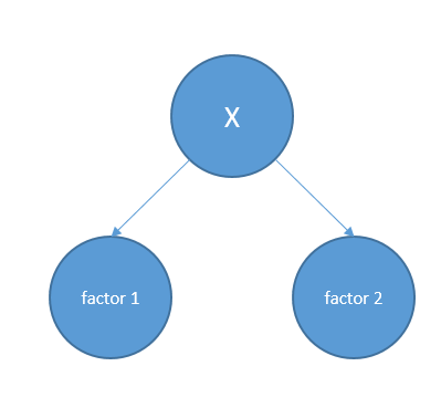
Having this model, factor1 and factor2 are dependent on each other. Because knowing factor1 can draw information about X and by having information about X, we would have information about factor2. But this contradicts with our independence assumption.
So we can rewrite it:
$ PDF_{noise}(x) = Normal(x, \mu , \sigma ) $
$ Y(x) = a.x + b + Noise $
Since there is a constant factor in the equation (b), without loss of generality, we can suppose the Normal Distribution has the mean equal to ZERO.
$ PDF_{noise}(x) = Normal(x, \mu=0 , \sigma ) $
Now, we want to find the most probable $ (a,b,\sigma)$ .
Now the probablity of Y is as follows:
$Y(x|a,b,\sigma) = a.X + b + Normal (0, \sigma^2) = Normal (a.X+b, \sigma^2 ) $
For finding the most probable configuration, we Use Maximum Likelihood Estimation.
Maximum Likelihood Estimation
Maximum likelihood estimation is a method used for finding the most likely parameters setting that can generate data samples. If we have m samples $(X_i, Y_i)$, and parameter $a, b $ then, we can calculate the probability of observation of data:
$ P (X,Y|a,b, \sigma) = \displaystyle\prod_{i=1}^{m} P(Y_i , X_i) = \displaystyle\prod_{i=1}^{m} P(X_i) P(Y_i | X_i) = \displaystyle\prod_{i=1}^{m} P(X_i) \displaystyle\prod_{i=1}^{m} P(Y_i | X_i) = $
$ \displaystyle\prod_{i=1}^{m} P(X_i) \displaystyle\prod_{i=1}^{m} Y(X_i|a,b,\sigma) = L1 * \displaystyle\prod_{i=1}^{m} Y(X_i|a,b,\sigma) $
We want to find $ (a,b,\sigma)$ that maximize the above likelihood. Since L1 is not a function of $ (a,b,\sigma)$ our parameters, we omit it and maximize the remaining part.
$ P (X,Y|a,b, \sigma) \propto \displaystyle\prod_{i=1}^{m} Y(X_i|a,b,\sigma)= \displaystyle\prod_{i=1}^{m} Normal (a.X_i+b, \sigma^2 ) = $
$ = \displaystyle\prod_{i=1}^{m} \frac {1}{\sqrt{2\pi\sigma}} \exp(- \frac{(x_i-\mu_{x_i})^2}{2 \sigma^2}) = (\frac {1}{\sqrt{2\pi\sigma}})^n \exp (\displaystyle\sum_{i=1}^{m} (- \frac{(x_i-\mu_{x_i})^2}{2 \sigma^2}) $
Logarithm Function is increasing in positive R so we will maximize $ log( P (X,Y|a,b, \sigma)) $ instead.
$ \log (P (X,Y|a,b, \sigma)) = -n \log (\sigma) + \displaystyle\sum_{i=1}^{m} (- \frac{(x_i-\mu_{x_i})^2}{2 \sigma^2}) = $
$ = -n \log (\sigma) + \frac {1}{2 \sigma^2} \displaystyle\sum_{i=1}^{m} - (x_i-{(a.x_i+b)})^2$
As we can see, for every $\sigma$, the maximum value of the above equation happens when the MSE is minimized.
So we can say this is one reason why it is meaningful to use MSE in a lot of different applications. At least when we want to use a linear regression model.
Conclusion
Using a probabilistic view, we tried to represent a reason why it is meaningful to use MSE in one specific task.
We can conclude that MSE is important because Central Limit Theorem is talking about normal distribution in which points with less quadratic distance to their mean are more probable.
So for further understanding, we can continue our story through the proof of Central Limit Theorem.